1-2 Geological Controls over the Earth’s Climate
For section 1-2 you should read Chapter 3 of the textbook and complete the exercises embedded in that chapter and then answer the questions at the end of Chapter 3.
As noted in section 3.1 of the textbook, understanding past changes in Earth’s climate is key to understanding anthropogenic (human-caused) climate change, and so we are going to review some of those changes in this section of the course. They have taken place, and continue to take place, on many different time scales, from billions of years to just minutes. Some of them are highly relevant to the processes of anthropogenic climate change; others are not. The geological controls over the Earth’s climate, and the history of our changing climate, are covered in Chapter 3 of the textbook. Please read that chapter, either before or while you are going through the material that follows here. If you aren’t familiar with the basic processes of climate change—such as how the greenhouse effect actually works, why albedo is important to climate, or the significance of climate feedbacks—you might want to read through Climate Change (Chapter 19) from the open textbook Physical Geology.
Past climate changes have been recorded in the geological record, in ancient rocks like those shown on Figure 3.0.1, or in relatively recent sediments on the sea-floor, or in glacial ice, or in the growth rings of trees, or the shells of living marine organisms. Earth scientists—with their experience in reading these types of records, their understanding of the geological processes that led to some of the important changes, and their appreciation for the vastness of geological time—are uniquely qualified to understand the history of Earth’s climate.
Solar and Atmospheric Evolution
As described in section 3.1 of the textbook, our sun, like all similar stars, is very slowly getting hotter, and sending more energy to the Earth (Figures 3.1.1 and 3.1.2). Over billions of years this increase in energy arriving on Earth would have led to a steady increase in the temperature on the Earth’s surface. However, that effect has been offset by the evolution of life, and the ability of life processes to change the composition of the atmosphere and hence the climate. Most of that change has been accomplished by taking carbon dioxide out of the atmosphere and storing it in the rocks of the Earth’s crust, so reducing the greenhouse effect. This process, and the biological changes that contributed to it, are illustrated on Figure 3.1.3. Note the (mostly) consistent slow decrease in the CO2 level over geological time, and relatively rapid rise of methane when life first evolved, and then the rapid decline of methane when the oxygen level started to increase.
There are two different types of processes that change our climate, forcings and feedbacks. The forcings are changes like the increase in greenhouse gas levels that is happening at present, while feedbacks are consequent changes that either strengthen the forcing (positive feedbacks) or suppress it (negative feedbacks). Box 3.2 in the textbook provides a summary of the important feedbacks that have played a role in past climate changes and are still operating today. Please take a close look at Table 3.1.1 and ensure that you understand how those feedbacks work.
Plate Tectonics and Climate
The various climate effects of plate tectonics are summarized in section 3.2 of the textbook. One of these is how the continents are situated on the globe because that can affect albedo and so lead to cooling.
• How does a concentration of continents near to the equator contribute to cooling?
• Why was that effect greater during the Proterozoic than it would be today?
A second effect is the construction of mountain chains, for the reasons already noted above, and a third is how plate tectonics can affect ocean currents. While we can predict with some confidence that a continental collision that produces a chain of mountains will lead to enhanced weathering and therefore consumption of atmospheric CO2 (and therefore to cooling), it is very difficult to predict how a future change in ocean currents resulting from a tectonic process might affect the climate, either on a local or a global scale. There are many ways in which ocean currents could be changed by tectonics in the future, and predicting how such changes might affect the climate is not straightforward.
The combined effects of mountain building and changes to ocean currents during the Cenozoic era are summarized on Figure 3.2.4. These processes have had a long-term cooling effect that has taken us from the hot-house of the Eocene era (ca. 55 Ma) to the ice-house of the Pleistocene era.
Volcanism and Climate
Volcanism can significantly affect the climate on both short and long time scales because volcanic eruptions add gases to the atmosphere. It is important to understand the message of Table 3.3.1 and the surrounding content because that will help you understand the role of volcanism in climate change.
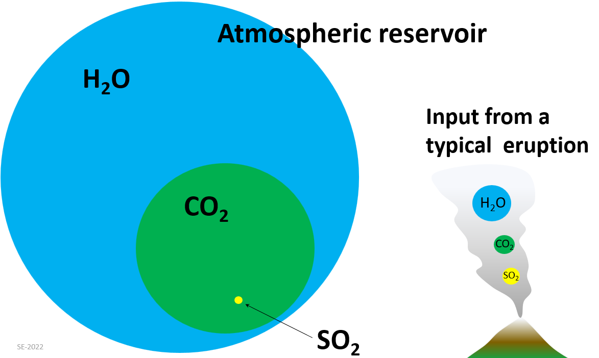
As is shown here on Figure 1-2, while a large volume of water is released during a volcanic eruption, it is a tiny amount compared with the amount of water already in the atmosphere. Furthermore, most of that volcanic water remains in the atmosphere for only days. Volcanic water has no effect on our climate.
A lot of CO2 is also released during an eruption, and while that is also small relative to the amount already in the atmosphere, CO2 can remain in the atmosphere for thousands of years, and so a long period of greater than average volcanism can result in a gradual but significant increase in the CO2 level, and eventually to warming.
In contrast, a single volcanic eruption can produce many times more SO2 than is typically stored in the atmosphere. That will have an immediate cooling effect because the SO2 gets converted to sulphate aerosols that block incoming sunlight. The effect will normally be short-lived because sulphate aerosols only stay in the atmosphere for a year or two.
The measured cooling effects of volcanic sulphate aerosols from three explosive eruptions in the 20th century are shown on Figure 3.3.1 in the textbook, and the modeled effects of CO2 warming and sulphate cooling for the massive Siberian Traps eruptions at around 250 Ma are shown on Figure 3.3.2.
Please complete Exercise 3.2 Volcanism and the Climate and then read section 3.4 of the textbook.
Orbital Variations and Climate
The Earth’s orbital and tilt variations are quite complex, and while you don’t need to understand them in detail, it is important to be aware of the following features:
- Our orbit around the sun is an ellipse (not a perfect circle) and the shape of that ellipse changes with time (Figure 3.4.1). When the orbit is most circular there is less potential for winter-summer extremes.
- The Earth is tilted relative to the plane of its orbit (Figure 3.4.2), and that tilt (which is what gives us our seasons) varies. The less tilt the less extreme the seasons.
- The direction of the tilt varies (the spinning Earth wobbles like a top) and the tilt direction determines which hemisphere (north or south) is farthest from the sun in summer.
The combination of these variations results in differences in the amount of solar heating at various latitudes on the Earth, and as described in the textbook, cool summers at high latitudes in the northern hemisphere promote the growth of glacial ice. This is especially so as the relatively cool summers would go on for thousands of years.
Since the insolation differences associated with the orbital variations are too small on their own to lead to a period of glaciation, what types of processes might play a role in leading the Earth into, or out of, a glacial cycle?
Ocean Currents and Climate
During the nearly 2.6 million years of the Pleistocene era, the Earth experienced a series of cold glacial periods and less-cold interglacial periods (like the one we’re in now). As shown on Figure 3.4.3, there is strong evidence that these variations were modulated by the orbital cycles, but it’s important to remember that these cycles did not cause the climate cooling that led to the glaciations of the late Cenozoic era. That can be attributed to the factors summarized on Figure 3.2.4. Orbital cycles have existed throughout the Earth’s history, and there is evidence that they have also influenced other aspects of the climate (e.g., monsoon variations).
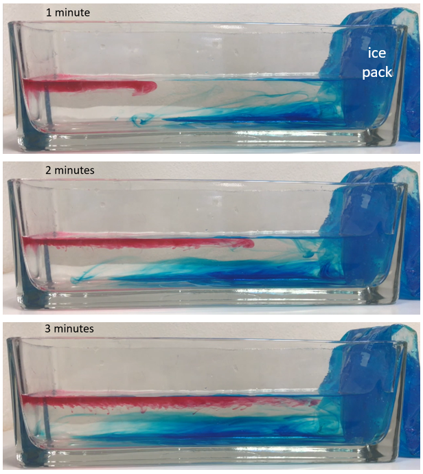
Ocean currents represent the most significant transportation of mass and thermal energy anywhere on Earth. The surface currents (Figure 3.5.1 in the textbook) are mostly driven by the winds (and so are powered by the sun), but the deeper currents (Figure 3.5.2) are powered by differences in water density, and so gravity is a driving force. Illustrated in Figure 3.5.5, seawater density differences are related to the salinity of the water (saltier water is denser than fresher water) and to the temperature of the water. Figure 1-3 shows the result of an experiment conducted with coloured water of different densities. You can easily do something like this at home with a teaspoon of salt, some hot and cold water, and a few drops of food colouring.
Exercise 1-1 Water Density Experiment
You can do something similar (but a little different) to what is shown on Figure 1-3 as follows:
- Fill a glass container with a volume of about 500 mL (a dish like the one in Figure 1-3, a drinking glass or glass jar) nearly to the top with room-temperature water. Add about 1/2 teaspoon of salt and stir well.
- In another small jar or glass, mix about 1 teaspoon of salt into about 50 mL of cold water from the tap (or from the refrigerator if your tap water isn’t cold). Add a couple of drops of blue food colouring. Stir well to dissolve the salt, but don’t worry if some of it won’t dissolve.
- Place about 50 mL of hot water (hot from the tap is sufficient) in another small jar or glass and add a couple of drops of red food colouring and stir.
- Gently pour about 20 mL of the blue salty water down the side of the larger jar. It should sink to the bottom and stay there.
- Lower a tablespoon of the hot red water into the water in the top part of the jar. It should stay near to the top, and the thermal and salinity stratification that you’ve created should last for some time, until the 3 types of water start to mix.
The salinity oscillator described on Figure 3.5.4 and the surrounding content is based on the principles demonstrated on Figure 1-3 (although no salt was used in that demonstration) and in the experiment above (Exercise 1-1). Salty water from the tropical part of the Atlantic sinks readily when it cools down in the far northern Atlantic, but if that water has been diluted by fresh water from melting glacial ice, the tendency to sink is reduced. The ~1500 year oscillation cycle is a function of how long it takes for glacial ice to build up during the cold parts of the cycle, and how long it takes before enough of that ice melts to dilute the Gulf Stream during the warm part.
Exercise 1-2 Visualizing Continental Positions
The following is an interactive version of Exercise 3.3 in the Environmental Geology textbook.
The density of ocean water is a function of its temperature and salinity, and the relationship is shown on the figure below, where density (red lines) is expressed in g/L. For example, at a salinity of 2.5% and a temperature of 10⁰ C, the density is 1027 g/L. The table has a list of salinities and typical water temperatures for some offshore locations, some within the Gulf Stream in the Atlantic and two within the Pacific. Point to those locations on the graph, and enter the density value provided in the table that follows.
| Location | Salinity (%) | T (° C) |
| North Carolina | 3.64 | 20 |
| Newfoundland | 3.58 | 15 |
| Iceland | 3.52 | 9 |
| Svalbard | 3.45 | 2 |
| Baja Sur | 3.4 | 20 |
| Los Angeles | 3.35 | 13 |
Extraterrestrial Impacts and Climate
Large extraterrestrial impacts are exceedingly rare on Earth, and, as far as we know, there has only ever been one—the K-Pg event— that caused intense climate effects and devastation to life. The important climate-change take-aways from section 3.6 of the textbook are that a large impact sends a vast amount of dust and gases into the atmosphere, and that can lead to immediate climate-cooling. Cooling also resulted from the smoke from intense, nearly global wildfires that followed the K-Pg impact. Also of note is that, depending on what type of rock is impacted (such as limestone in the case of the K-Pg impact), the cooling could be followed by greenhouse warming (CO2 from the CaCO3 of the limestone), which in this case is modelled to have lasted about 100,000 years.
• How might the result of the K-Pg event have differed if the impact had taken place in an area with crystalline rocks like those of the Canadian Shield, rather the the sulphate- and carbonate-bearing rocks of the Chicxulub region of Mexico?
• How might the result have been different if the event had taken place 500 million years ago, when there was almost no vegetation on the land?
