4-3 Water Resources

Iceland’s Gullfoss waterfall, shown on Figure 11.0.1 in the textbook, is fed largely from the melting of the Langjukoll Glacier, which, like most glaciers in Iceland, and everywhere else, is retreating rapidly with climate change. The melting leading to that retreat makes the falls spectacular now, but it is inevitable that the ongoing loss of ice will lead to a future of lower flows on this and other Icelandic rivers. While that might not have significant implications for thinly populated Iceland, it is a big problem for many other parts of the world where municipal water supplies rely on summertime melt of glaciers and snowpacks to keep rivers flowing and/or reservoirs sufficiently full. Some cities that come to mind include Vancouver, Victoria, Calgary, and Edmonton in Canada, and Seattle, Tacoma, and Portland in the Pacific Northwest and many other cities in the US close to mountainous terrain. Climate warming is putting some of these water supplies at risk, and changes in precipitation patterns are creating problems for water supplies in many other places as well, including Cape Town, South Africa (Figure 11.0.2 in the textbook).

Section 11.1 covers the paces where water is stored on Earth, what proportion is stored in each of those “reservoirs”, and how long a typical molecule of water will remain in one of those reservoirs. That’s important, so please complete Exercise 4-4 below.

It’s easy to think of growing food as a wholesome and healthy activity that we all benefit from, but modern mechanized and chemical-intensive farming methods are changing that. Agriculture is the main source of water contamination in areas with intensive agriculture, partly because of the use of pesticides and herbicides (see Figure 11.2.1 in the textbook), partly because of the wide use of fertilizers (Figure 11.2.2), and commonly just because cultivated fields are prone to erosion (Figure 11.2.3).

Of course, farming isn’t the only activity that is polluting our water sources. Industry plays a major role, although tightening regulations are helping with that. Forestry is significant, especially with regard to increasing levels of suspended sediment in surface waters, which has both human and environmental impacts. As noted above, mining and other resource extraction can negatively affect water sources, but our continuing use of fossil fuels also has a significant impact because we tend to be careless about how fuels are transported and stored (see Figures 11.2.6 and 11.2.7).

Section 11.3 of the textbook covers the topic of natural effects on water quality. For the most part this has to do with water being in contact with sediments and rocks, and the consequent water-mineral interactions changing the dissolved composition of the water. An important point is that it doesn’t necessarily take high concentrations of an element in the rock or sediment to result in elevated concentrations in the water. This is illustrated by the elevated levels of fluoride in Nanaimo area groundwater (Figure 11.3.5 and related text), and also by the elevated levels of arsenic in shallow groundwater in Bangladesh (Figure 11.3.6 and related text).

Another important contamination issue is intrusion of saltwater in areas near to ocean shores. As described in the textbook, we can expect that problem to get worse in coming years because of climate change and sea-level rise.

Groundwater is discussed in section 11.4 of the text. As summarized on Table 11.1.1 (back in section 11.1), about 60 times more fresh water is stored in the ground (in aquifers) than in all of the lakes and rivers on the surface. On the other hand, water moves very slowly through aquifers (hence the 300-year average residence time) and that has to be taken into account when we consider using groundwater as a source. The flow volume of groundwater is not much higher than the flow volume of rivers, and therefore it is easy to deplete an aquifer if we overuse it.

Aquifers are made up of either unconsolidated sediments (gravel, sand silt for example) or solid rock. The important properties of these materials are their porosity (how much water they can hold) and their permeability (how easily water will flow through them). These are illustrated on Figure 11.4.1 and 11.4.2 in the textbook. Permeability is the critical parameter from the perspective of water supply.

It is important to recognize that surface water (water in streams and lakes) and groundwater are not separate entities, they are the same water in different places, and as illustrated on Figure 11.4.4 there is ongoing interchange between the two. Surface water moves down through soil, sediment and rock to become groundwater, and groundwater is discharged to become surface water.

An aquifer is a body of rock or sediment that is saturated with water and that has sufficient permeability to supply water, typically via a well. As shown on Figure 11.4.4, the upper surface of the zone of saturation is the water table. Many people misunderstand the term “water table”.  A water table isn’t a physical object, and it isn’t a body of stored groundwater; it is just the upper limit of the saturated zone of an aquifer. We extract water from an aquifer, not from a water table. The water table varies significantly, in that it will be higher during wet parts of a year and lower when it is dry. If you drill a well into an aquifer the well will be full of water up to the level of the water table. This is illustrated on Figure 11.4.5, but it only applies to unconfined aquifers (although that includes most aquifers); Well A is drilled into an unconfined aquifer and the top of the water in the well coincides with the water table.

A confined aquifer is a permeable body (of sediment or rock) that is overlain by a layer of material that is relatively impermeable. In Figure 11.4.5 the values of K denote permeability. The confined aquifer (with K = 10-2) is 10,000 times more permeable than the confining layer (K = 10-6). Water percolating down from surface is effectively stopped by the confining layer, and so the only way for a significant amount of water to get into the confined aquifer is where it is exposed at surface (upper left). The confined aquifer has its own “water table” but it is known as a potentiometric surface.

Figure 11.4.7 shows likely water flow paths within an aquifer. The flow paths are determined by the shapes of the water-pressure contours (equipotential lines). That means that the water flow isn’t necessarily vertical just below the water table, and that in some places (e.g., near to a discharge area) it can flow “up hill”.

As illustrated on Figure 11.4.8, we can estimate the rate of groundwater flow between any two points if we know the permeability and porosity of the aquifer and the gradient of the water table between those points. Please make sure you understand how to do this by completing Exercise 11.3 Groundwater Flow Rate.

Section 11.5 of the textbook covers streams and stream flow, including the concepts of a drainage basin (the land area from which water flows to form a stream; see Figure 11.5.1), variations in the gradient of a stream (Figure 11.5.3) and variations in the discharge (hydrograph) of a stream over a year (Figure 11.5.4). Streams in different climates and environments have widely differing hydrographs, depending on the seasonality of precipitation, variations in temperature, and the significance of snow accumulation (and glaciers), which are dependent on topography and climate.

Stream ecosystems have evolved to fit within the flow characteristics of the stream hydrograph, and humans have created stream water-supply and energy systems that depend on those flow characteristics. Other human infrastructure, such as roads and bridges, also depend on understanding stream discharge characteristics.

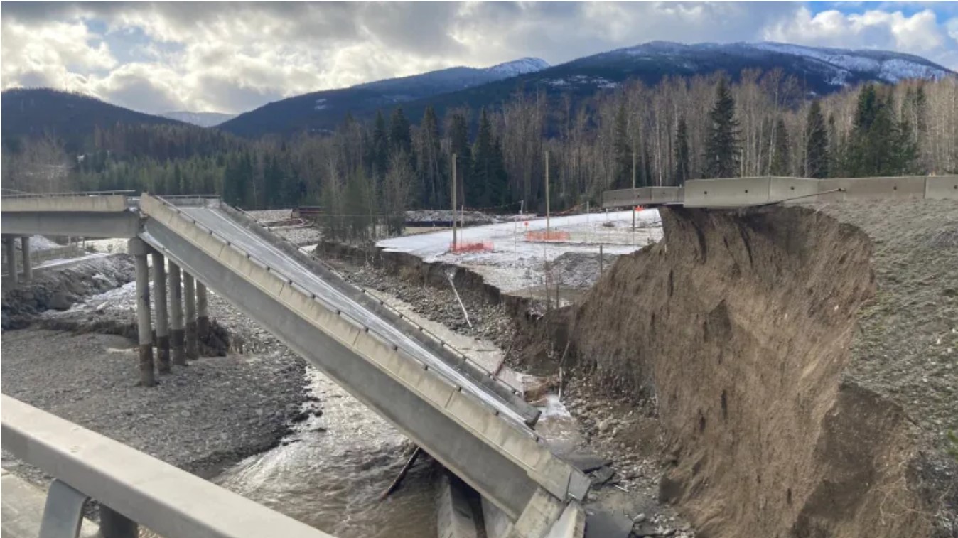
Climate change is upsetting some of these systems. For example, as mentioned above, climate change has made some areas drier and most areas warmer, so that water supplies for humans and ecosystems are challenged. Climate change has also led to more variable weather in most regions, and this is exemplified by the situation shown on Figure 4-4 below. Unusually intense rainfall in southern British Columbia in November 2021 led to stream flow levels that had not been anticipated by the engineers that designed roads, railways and bridges. These designs were based on past flood level data, not on projections of floods that might occur with climate change.